


In Part 1, we looked at SMT solvers. Their natural question is whether a carefully constructed set of constraints can be satisfied. That is enough to prove many local facts about a system: a counter cannot become negative in one step, an unauthorized transition cannot be enabled, or a proposed invariant is preserved by each rule.
But many requirements are not about one state or one step. They are about what happens over time.
A controller may be safe now and fail later. A request may be accepted but never completed. Recovery may remain possible without ever being taken. To discuss those differences, formal verification needs a language for executions.
That is the natural territory of temporal model checking.
An LTL or CTL model checker asks a question of the following shape:
Does this transition system satisfy this required pattern of behavior?
This is a major increase in scope. The checker reasons about whole futures, often across a state space far larger than anyone would inspect manually. Yet temporal logic is still an observation language with a defined point of view. It makes some distinctions precise and leaves others outside its native view.
A proof assistant changes the level again. It can define the transition system, define executions as formal objects, and state custom relationships among several executions. The difference is not that it has one more temporal operator. It is that the objects being observed by temporal logic can themselves become objects of proof.
The running controller, now viewed through time
We continue with the safety controller introduced in Part 1. It receives commands, checks permissions and interlocks, drives an actuator, records audit information, and enters recovery after certain faults.
A state may record:
- the current mode;
- the active command;
- queue contents;
- permission and interlock bits;
- watchdog and retry counters;
- pending acknowledgements.
A transition applies one controller rule. The resulting graph contains every state that the model allows and every step between them.
The requirements now concern complete behavior:
The controller never enables the actuator while an interlock is open.
Every accepted request is eventually acknowledged.
From every fault state, recovery remains possible.
The controller cannot perform internal work forever while ignoring an accepted command.
These are not merely larger Boolean formulas about one snapshot. They concern ordering, possibility, inevitability, and repetition across executions.
Two temporal viewpoints
LTL and CTL organize those questions differently.
Linear-time temporal logic (LTL) describes patterns along an execution. Its best-known operators have intuitive readings:
- always: a condition holds from now on;
- eventually: a condition will hold at some later point;
- until: one condition continues until another occurs.
For example, a response requirement can be written schematically as:
always (request implies eventually acknowledgement)
In standard notation:
G(request -> F acknowledgement)
SPIN, for example, accepts LTL requirements and checks a model for counterexamples to them.1
Computation tree logic (CTL) makes branching choices explicit. It can distinguish statements such as:
- from a state, some future reaches recovery;
- from a state, every future reaches recovery;
- from every reachable state, there exists a route back to service.
The syntax matters in real verification work, but the mental distinction is more important here:
LTL describes patterns along executions. CTL combines temporal patterns with explicit choices over possible futures.
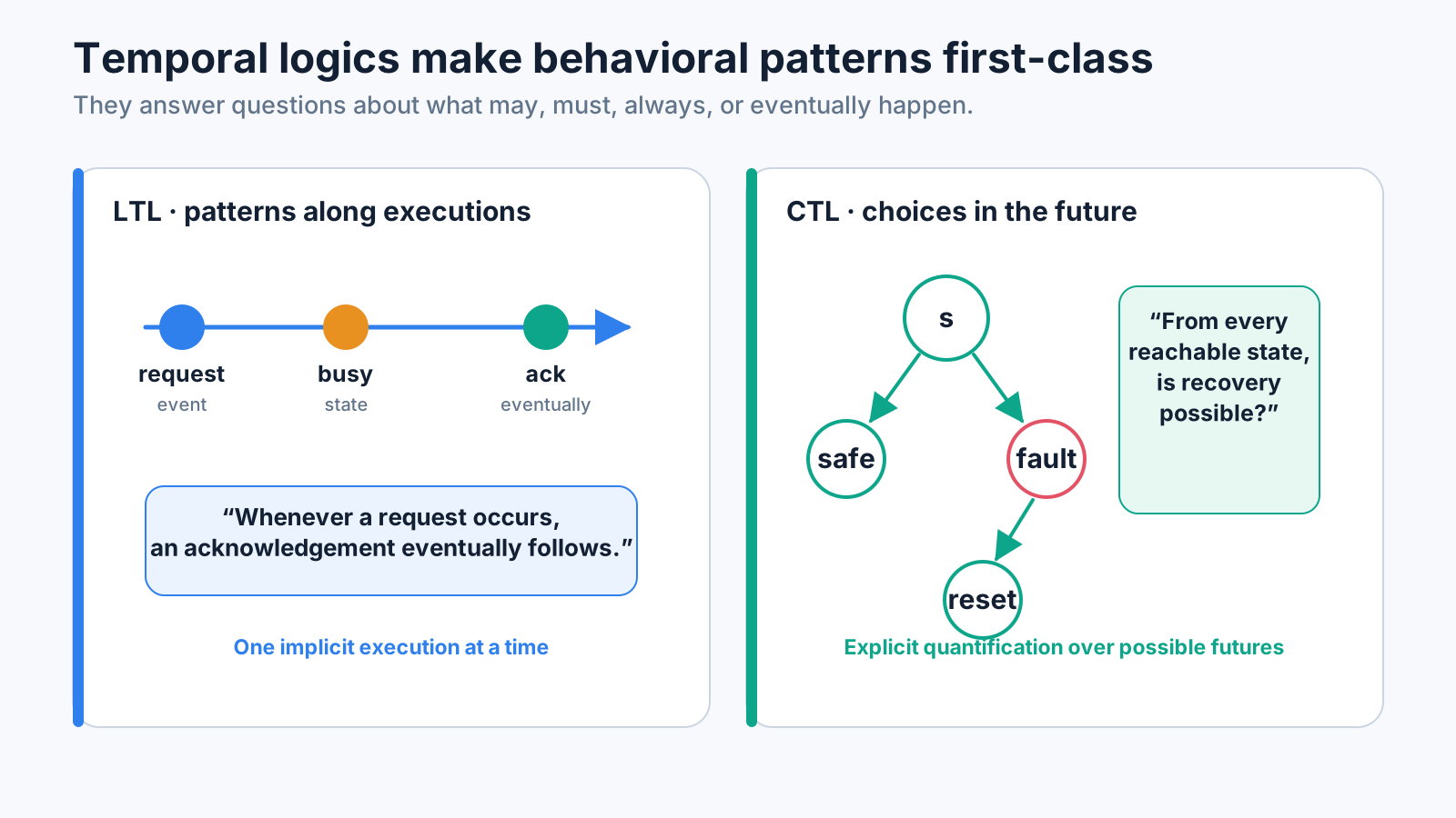
Both logics turn time into something a checker can analyze automatically. They support properties far beyond one-step constraints.
What the checker gives us
For a finite-state model, a temporal model checker can often answer the property automatically.
If the property holds, the result is a global statement about all relevant behavior of the model. If it fails, the checker usually produces a counterexample path or a related diagnostic structure.
For the request–acknowledgement property, a counterexample might look like:
request
work
retry
work
retry
work
...
The value of this result is difficult to overstate. A single execution can expose a missing fairness assumption, an unhandled scheduler choice, a forgotten timeout transition, or a genuine liveness failure.
Temporal model checking also benefits from decades of specialized algorithms: symbolic state representations, automata constructions, partial-order reduction, fixpoint computation, and on-the-fly search. As with SMT, the restriction of the specification language is not an accidental weakness. It is part of what makes strong automation possible.
Mental model: A temporal model checker observes the transition system through a fixed language of behavioral patterns.
What does the observation language see?
To evaluate a temporal formula, the model exposes observations about states—propositions such as:
request_pending
unsafe
fault
recovered
The logic follows paths through the graph and observes how those propositions change.
This means that two different internal state graphs may look the same to the logic when they produce the same relevant observations. In many applications that is desirable. Verification should ignore implementation details that do not affect the requirement.
But it also means that temporal equivalence is not the same thing as structural identity.
That distinction becomes visible in our recurring reconvergence example.
Two systems that look the same over time
Consider two small transition systems.
In the joined system, an initial state has two possible branches. Both branches later reach the same state.
In the split system, the initial state also has two branches. Each reaches a separate copy of the final behavior. The copies have the same labels and make the same future moves, but they are not one shared state.
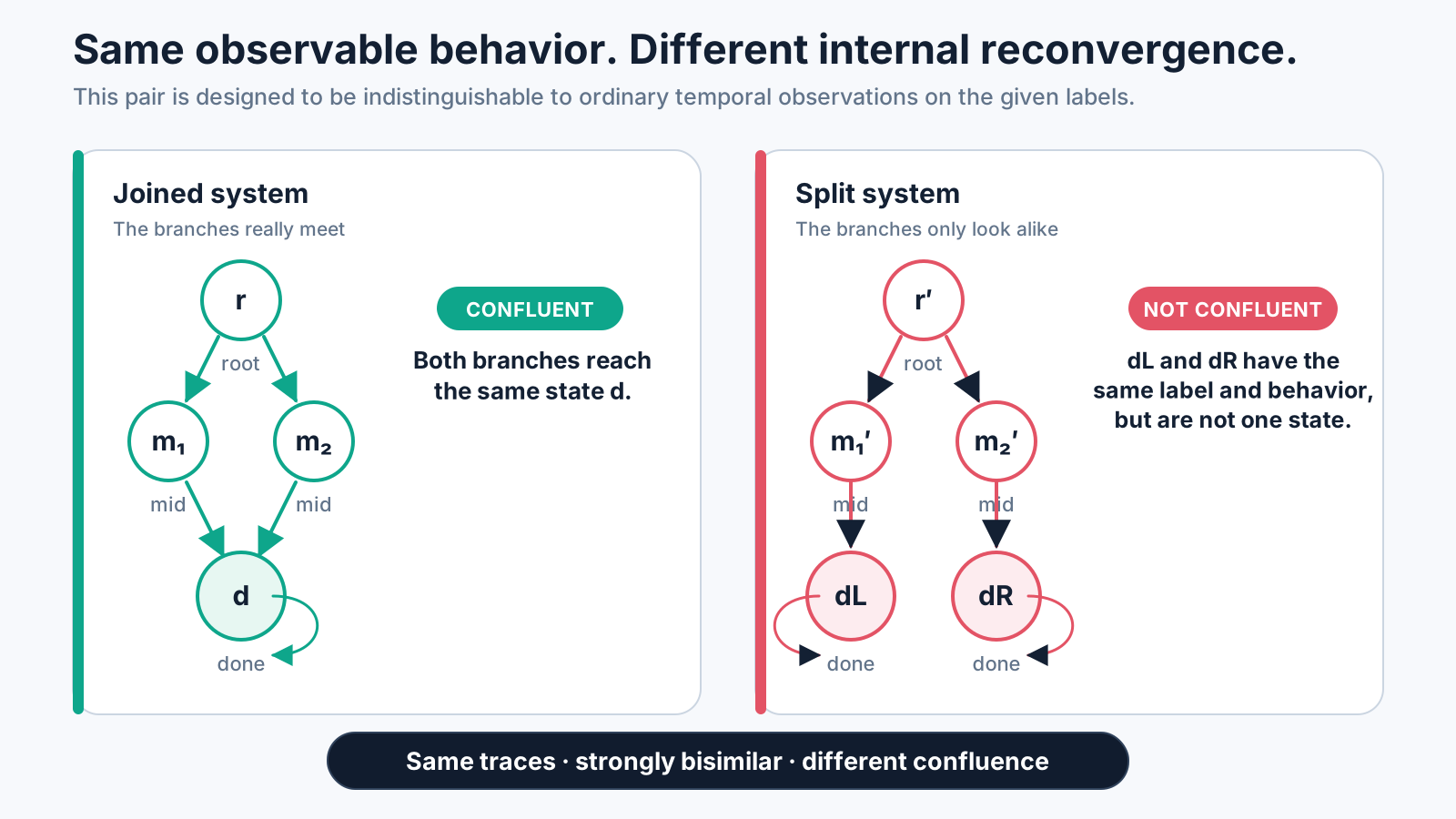
From an external viewpoint, both systems show the same sequence of observations:
root, mid, done, done, done, ...
Suppose their corresponding transitions also carry the same action names. Each move in one system can then be matched by a move in the other, and the resulting states remain behaviorally related. In the standard terminology, the two initial states are strongly bisimilar.
Strong bisimulation is an intentionally demanding behavioral equivalence: matching states must be able to match each other’s actions step by step. Even so, it does not require the two branches inside one model to end at literally the same state.
The joined system has the property we have been calling reconvergence, or confluence:
Whenever two finite executions begin in the same state, their endpoints can later reach a common state.
The split system does not. Its two middle states enter separate components and never share a descendant.
Yet no ordinary CTL* formula over the given state labels can distinguish the two initial states. CTL* formulas are invariant under the relevant notion of bisimulation; for finite Kripke structures, the classical characterization by Browne, Clarke, and Grumberg makes this connection precise.2
LTL cannot distinguish this pair either because the labelled traces are the same.
The important conclusion is not “temporal logic is too weak.” It is more specific:
A logic that observes labelled temporal behavior need not expose whether two behaviorally identical branches later occupy the identical underlying state.
That is a different kind of fact about the transition structure.
The scope of the expressibility claim
Statements about what a model checker “cannot express” require care.
For this series, native expressibility means:
One fixed formula is interpreted over the original model and its original observations, without first adding unique state labels, computing a reachability relation, constructing a product model, or changing to a richer logic.
Under that convention, the joined and split systems establish a clean boundary: a CTL*, CTL, or LTL formula cannot characterize confluence on the original labelled systems, because the property differs between systems that the logic cannot distinguish.
This does not imply that temporal-model-checking technology can never participate in checking confluence. A verification engineer might:
- instrument the model with additional state identity;
- construct an observer or product system;
- encode pairs of paths;
- use a fixed-point, relational, or hyperproperty logic;
- exploit a finite bound;
- reduce a specialized confluence criterion to ordinary safety.
Those are legitimate techniques. They enlarge or transform the question.
The distinction to preserve is:
Native formula over the original model is not the same as checkable after a suitable reduction.
Without this distinction, comparisons among formal verification tools quickly become misleading. With unrestricted preprocessing, the front end may do most of the semantic work before the checker ever sees the problem.
A proof assistant can make paths into objects
In a proof assistant, the transition graph is not only something an algorithm traverses. We may define finite paths explicitly.
Conceptually, a path from state s to state t contains:
- either evidence that
sandtare the same state, representing zero steps; - or one valid transition followed by a shorter path.
The confluence statement can then refer to two particular path objects:
Given a path from a to b
and a path from a to c,
produce a state d,
a path from b to d,
and a path from c to d.
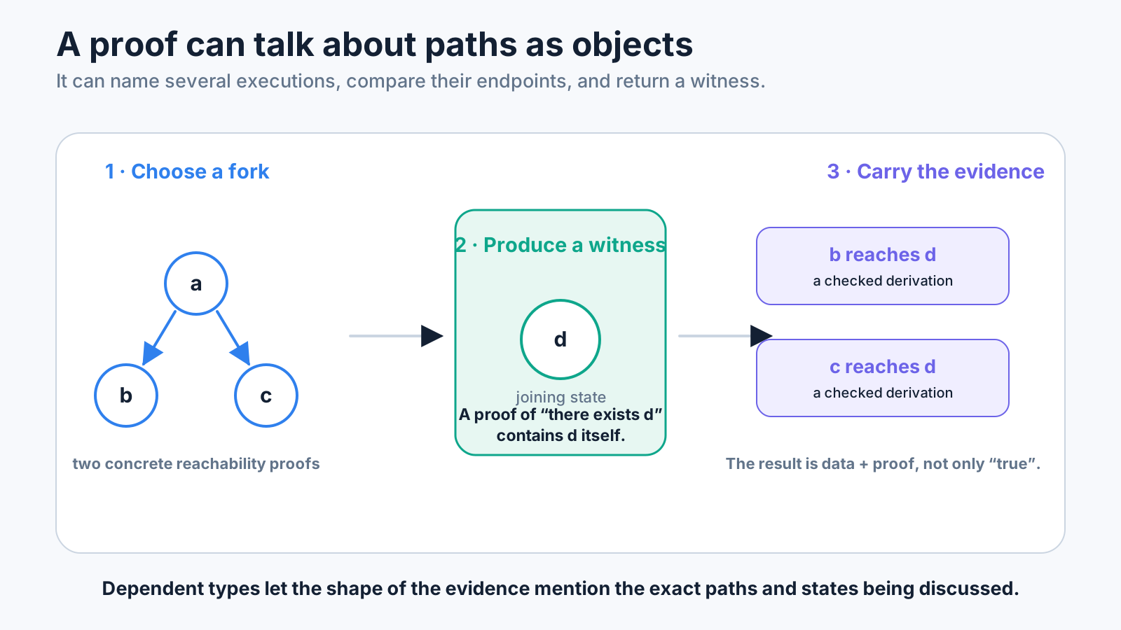
This illustrates a small but important idea from dependent type theory:
A proof may contain a witness, and the type of the accompanying evidence can mention that exact witness.
The result is more informative than a bare true value. It can contain the joining state and the two checked derivations showing that it is reachable from both branches.
The proof assistant can also express variations without waiting for a logic designer to add new primitive operators:
- the branches reach the identical state;
- the branches reach equivalent states;
- one branch simulates the other;
- the paths agree on low-security observations;
- the branches reconverge within a resource bound;
- reconvergence holds only under a scheduler assumption.
Each version is a different theorem because each captures a different engineering requirement.
This is where dependent types matter
The phrase dependent type can sound more difficult than the idea needed here.
An ordinary type might say:
this object is a State
A dependent type can say:
this object is evidence that this particular state reaches that particular state
The endpoints are part of the claim’s type. A proof cannot silently substitute an unrelated path without being rejected.
Across Agda, Lean, and Rocq, the details differ, but this broad type-theoretic pattern is common:3
- executions can be represented by inductive families;
- propositions can mention concrete values;
- a proof can carry witnesses;
- induction over a path mirrors its construction.
The point for a non-specialist is architectural. The language is not limited to a fixed catalogue of temporal operators. Users can define the semantic objects and relationships that their assurance argument requires.
What proof might look like—without teaching proof scripts
How would someone actually prove confluence for the controller?
One route is to establish a local fact:
Whenever two different rules are both enabled in the same state, applying either one first leads to states that can be joined.
The proof may divide rule pairs into cases:
- the rules modify independent fields and commute immediately;
- one rule disables the other but both orders reach an equivalent state;
- a priority rule resolves the conflict;
- the pair is impossible because their guards are inconsistent.
SMT can be valuable inside these cases. It may prove that two guards cannot be true together or that two updates produce equal data.
A second theorem can then lift local reconvergence to arbitrary finite executions, perhaps using termination or another global condition. The Isabelle Archive of Formal Proofs, for example, contains a reusable formalization of abstract rewriting with confluence, joinability, normalization, and Newman’s lemma.4
This is the hybrid pattern again:
- temporal model checking handles temporal properties in its native language;
- SMT discharges local data obligations;
- the proof assistant states and checks the larger semantic theorem.
LLMs can help construct relational proofs
The formal work becomes more demanding as soon as a theorem mentions several executions. Useful intermediate statements are not always obvious.
An LLM can propose:
- a relation that should remain invariant between two paths;
- a case split over pairs of transition rules;
- a local diamond or commutation lemma;
- an induction over a path derivation;
- a library theorem that connects local and global confluence;
- solver calls for arithmetic side conditions.
The proof assistant still checks every accepted definition and proof term. The LLM does not become the logical authority.
This feedback loop is especially valuable because relational proofs contain many opportunities for small mismatches: the wrong endpoint, a reversed relation, an assumption available on only one branch, or a lemma stated at the wrong level of generality. A type checker can reject these errors precisely.
The same limitation from Part 1 remains. The proof assistant verifies consequences of the formal model. It does not guarantee that labels such as unsafe or acknowledgement were defined correctly with respect to the deployed controller. Model validation remains a central engineering task.
The mental map after Part 2
| Question | Natural home |
|---|---|
| Is an unsafe state reachable? | Temporal model checker, reachability checker, or SMT-based bounded analysis |
| Does every request eventually receive an acknowledgement? | LTL or another temporal logic |
| From every fault state, is some recovery path available? | CTL or another branching-time logic |
| Do two named executions reach the same state? | Relational semantic statement |
| What exactly is an execution, endpoint, or joining witness? | Proof-assistant definition |
| Can temporal results become premises in a larger theorem? | Proof-assistant composition |
Temporal model checking is not merely “SMT with more steps.” It gives time and branching their own specification languages and algorithms. That specialization is why it works so well.
A proof assistant does something complementary:
It lets us reason not only through a temporal language, but also about the model, the executions, the observation scheme, and the meaning of the temporal result.
Part 3 moves from properties to abstraction. Refinement and equivalence checkers compare one behavioral model with another. They come closest to the idea of layered verification—but every comparison relation preserves only selected distinctions.
Sources and further reading
-
SPIN documentation, “Linear Time Temporal Logic Formulae”. The reference describes SPIN’s
always,eventually,until, and related LTL operators and its counterexample-oriented checking workflow. ↩︎ -
M. C. Browne, E. M. Clarke, and O. Grumberg, “Characterizing Finite Kripke Structures in Propositional Temporal Logic”, Theoretical Computer Science 59, 1988. The paper relates finite-state temporal equivalence and a bisimulation-style structural equivalence and proves preservation of CTL* formulas. ↩︎
-
Lean documentation, “Inductive Types” in Theorem Proving in Lean 4. The chapter explains inductive types, inductively defined propositions, dependent families, and the associated induction principles. ↩︎
-
Christian Sternagel and René Thiemann, “Abstract Rewriting”, Archive of Formal Proofs. The development formalizes reachability, joinability, confluence, normalization properties, and results including Newman’s lemma. ↩︎